---
title: "Reanalysis of an ALS Gut Microbiome with DeepTaxa"
subtitle: "DADA2 ASVs, DeepTaxa classification, validation against SILVA, and a paired ALS versus control comparison"
keywords: [16S rRNA, amplicon sequence variants, DeepTaxa, taxonomic classification, gut microbiome, amyotrophic lateral sclerosis, DADA2, SILVA]
format:
html:
toc: true
toc-depth: 3
toc-title: "Contents"
code-fold: show
code-tools: true
number-sections: true
fig-cap-location: bottom
theme: lumen
execute:
warning: false
message: false
echo: true
---
This notebook is the technical companion to the case study. It documents the complete
pipeline for reanalyzing a published amyotrophic lateral sclerosis (ALS) gut-microbiome
16S rRNA dataset with DeepTaxa, and it reproduces every figure and statistic from the
committed data. The upstream steps (read download, amplicon sequence variant inference, and
classification) are given as documented code and runnable scripts; the ALS versus control
analysis runs at render time from the amplicon sequence variant (ASV) table and the
taxonomy tables that ship with this repository.
Because these are 16S V4 reads, the analysis uses the DeepTaxa checkpoint, which is
trained for that region. After classification, we test whether the high-confidence genus
calls are also correct by comparing DeepTaxa against an independent SILVA classification of
the same ASVs, and then carry out the paired clinical comparison.
# The dataset
The data are 18 sequencing runs from a study of the gut microbiome in ALS, in which each
patient was paired with their spouse as a control so that cases and controls share diet,
household, and environment. The runs are 16S rRNA **V4** amplicons (515F/806R primers,
about 250 to 254 base pairs after merging), sequenced on an Illumina MiSeq. They
represent 9 of the study's 10 matched pairs; one pair was not deposited.
| Pair | ALS | Control |
|------|-----------|-----------|
| 1 | [SRR10153501](https://www.ncbi.nlm.nih.gov/sra/SRR10153501) | [SRR10153511](https://www.ncbi.nlm.nih.gov/sra/SRR10153511) |
| 2 | [SRR10153503](https://www.ncbi.nlm.nih.gov/sra/SRR10153503) | [SRR10153499](https://www.ncbi.nlm.nih.gov/sra/SRR10153499) |
| 3 | [SRR10153500](https://www.ncbi.nlm.nih.gov/sra/SRR10153500) | [SRR10153504](https://www.ncbi.nlm.nih.gov/sra/SRR10153504) |
| 5 | [SRR10153502](https://www.ncbi.nlm.nih.gov/sra/SRR10153502) | [SRR10153505](https://www.ncbi.nlm.nih.gov/sra/SRR10153505) |
| 6 | [SRR10153509](https://www.ncbi.nlm.nih.gov/sra/SRR10153509) | [SRR10153514](https://www.ncbi.nlm.nih.gov/sra/SRR10153514) |
| 7 | [SRR10153507](https://www.ncbi.nlm.nih.gov/sra/SRR10153507) | [SRR10153512](https://www.ncbi.nlm.nih.gov/sra/SRR10153512) |
| 8 | [SRR10153510](https://www.ncbi.nlm.nih.gov/sra/SRR10153510) | [SRR10153508](https://www.ncbi.nlm.nih.gov/sra/SRR10153508) |
| 9 | [SRR10153506](https://www.ncbi.nlm.nih.gov/sra/SRR10153506) | [SRR10153515](https://www.ncbi.nlm.nih.gov/sra/SRR10153515) |
| 10 | [SRR10153513](https://www.ncbi.nlm.nih.gov/sra/SRR10153513) | [SRR10153573](https://www.ncbi.nlm.nih.gov/sra/SRR10153573) |
: Sample pairing. Nine ALS patients, each matched to a spouse control. {#tbl-samples}
The dataset was published by @hertzberg2021als, BioProject [PRJNA566436](https://www.ncbi.nlm.nih.gov/bioproject/PRJNA566436). This is a
reanalysis of that cohort with an independent classification method.
# Reproducing the inputs
The analysis below runs from the ASV table and the taxonomy tables committed under
[`data/`](https://github.com/systems-genomics-lab/deeptaxa/tree/main/tutorials/casestudy/data), so the notebook reproduces without rerunning anything upstream. Those inputs are
themselves reproducible from the public raw reads: the 18 runs are on the Sequence Read
Archive, with the run accessions in the first column of [`data/samples.tsv`](https://github.com/systems-genomics-lab/deeptaxa/blob/main/tutorials/casestudy/data/samples.tsv) (and in
@tbl-samples). The steps are summarized below; the runnable scripts for the compute-heavy
parts and the full tool versions are in [`pipeline/`](https://github.com/systems-genomics-lab/deeptaxa/tree/main/tutorials/casestudy/pipeline).
The raw reads are fetched with the SRA Toolkit:
```{#lst-fetch .bash lst-cap="Fetch the raw reads from the SRA with the SRA Toolkit."}
# For each run accession in the sample sheet: download, split into paired FASTQ, and compress.
for s in $(tail -n +2 data/samples.tsv | cut -f1); do
    prefetch "$s"
    fasterq-dump "$s" --split-files -e 4
    pigz "${s}_1.fastq" "${s}_2.fastq"
done
```
## ASV inference (DADA2)
The raw paired-end reads were denoised into ASVs with DADA2 1.40.0. DADA2 performs its own
quality filtering [@callahan2016dada2], so no separate trimming step is used on this route:
it filters each read to an expected-error budget of 2 with no length truncation, learns the
error model, denoises with pseudo-pooling, merges the read pairs, and removes chimeras. Of
229,204 input
read pairs, 99.8 percent passed filtering and 178,378 (77.8 percent) survived as
non-chimeric reads, yielding **276 V4 ASVs**. The full script is [`pipeline/01_dada2_asv.R`](https://github.com/systems-genomics-lab/deeptaxa/blob/main/tutorials/casestudy/pipeline/01_dada2_asv.R).
```{#lst-dada2 .r lst-cap="Denoise the reads into ASVs with DADA2: filtering, error learning, pair merging, and chimera removal."}
filterAndTrim(fnF, filtF, fnR, filtR, truncLen = 0, maxN = 0, maxEE = c(2, 2),
              truncQ = 2, minLen = 50, rm.phix = TRUE, multithread = TRUE)
ddF <- dada(filtF, err = learnErrors(filtF), pool = "pseudo")   # and the reverse reads
seqtab <- removeBimeraDenovo(makeSequenceTable(mergePairs(ddF, filtF, ddR, filtR)),
                             method = "consensus")               # 276 ASVs
```
## Taxonomic classification (DeepTaxa and SILVA)
The ASVs were classified with the DeepTaxa checkpoint [@salah2026deeptaxa], which is
trained for the V4 region these reads cover. On these amplicons it assigns a genus to 99
percent of reads at high
confidence (mean 0.985). DeepTaxa inference is deterministic; re-running it yields a
byte-identical taxonomy.
```{#lst-predict .bash lst-cap="Classify the ASVs with DeepTaxa."}
deeptaxa predict --fasta-file asv_seqs.fasta --checkpoint deeptaxa-v4-v2.pt \
  --output-dir out --tabular --batch-size 128 --num-workers 4
```
The checkpoint is published at
[huggingface.co/systems-genomics-lab/deeptaxa](https://huggingface.co/systems-genomics-lab/deeptaxa),
and the tabular output (`out/asv_seqs_deeptaxa_predictions.tsv`) is committed as
[`data/asv_taxonomy.tsv`](https://github.com/systems-genomics-lab/deeptaxa/blob/main/tutorials/casestudy/data/asv_taxonomy.tsv). High confidence reflects how well the
input matches the model's training regime and is not by itself evidence of correctness, so
the same ASVs were also classified independently with the SILVA v138 reference
[@quast2013silva] ([`pipeline/02_classify_silva.R`](https://github.com/systems-genomics-lab/deeptaxa/blob/main/tutorials/casestudy/pipeline/02_classify_silva.R)) as a cross-check.
# Setup and data loading
All sections below execute from the committed files.
```{python}
#| lst-label: lst-setup
#| lst-cap: "Load the sample sheet, ASV count table, and DeepTaxa taxonomy, and align them."
import numpy as np, pandas as pd
from scipy import stats
import matplotlib.pyplot as plt
import re

# The seven taxonomic ranks DeepTaxa predicts, ordered from broadest to finest.
RANKS = ["domain","phylum","class","order","family","genus","species"]
CONF = 0.5                        # minimum confidence for a taxonomic call to be counted
rng  = np.random.default_rng(42)  # fixed seed, so the permutation tests are reproducible
colors = {"ALS":"#d1495b","Control":"#30638e"}

# Sample sheet: one row per run, carrying its ALS/Control status and pair number.
meta   = pd.read_csv("data/samples.tsv", sep="\t")
pairs  = meta.pivot(index="pair", columns="status", values="sample").dropna()  # pair -> ALS, Control
als    = meta.loc[meta.status=="ALS","sample"].tolist()
ctl    = meta.loc[meta.status=="Control","sample"].tolist()

# Count table (ASVs x samples) and the per-ASV taxonomy, kept in the same ASV order.
counts = pd.read_csv("data/asv_counts.tsv", sep="\t", index_col=0)
tax    = pd.read_csv("data/asv_taxonomy.tsv", sep="\t").set_index("sequence_id")
counts = counts.loc[tax.index]              # align the count table to the taxonomy rows
rel    = counts / counts.sum(axis=0)        # convert counts to per-sample proportions
reads  = counts.sum(axis=1)                 # total reads per ASV, used for read-weighting

print(f"{counts.shape[0]} ASVs, {counts.shape[1]} samples; "
      f"{len(als)} ALS and {len(ctl)} control, {len(pairs)} matched pairs")
```
# Validation against SILVA
The SILVA classification of the same ASVs provides an independent check on the DeepTaxa
genus calls. Because DeepTaxa reports GTDB names and SILVA reports NCBI names, genus labels
are harmonized (GTDB suffixes removed, a small set of documented synonyms mapped) before
comparison.
```{python}
#| lst-label: lst-concordance
#| lst-cap: "Harmonize DeepTaxa (GTDB) and SILVA (NCBI) genus names and measure their agreement."
sv = pd.read_csv("data/asv_taxonomy_silva.tsv", sep="\t").set_index("ASV")

# Documented GTDB-to-NCBI genus synonyms, so equivalent genera are not scored as disagreements.
SYN = {"limosilactobacillus":"lactobacillus", "shigella":"escherichia",
       "phocaeicola":"bacteroides", "mediterraneibacter":"ruminococcus"}

def base_genus(x):
    """Reduce a genus label to a bare, lower-case name: drop GTDB suffixes (Blautia_A -> blautia),
    take the first token, then map through the synonym table. Returns None for missing values."""
    if not isinstance(x, str) or x.strip() in ("","NA","nan"): return None
    g = re.sub(r"_[A-Za-z0-9]+", "", x).split()[0].lower()   # strip GTDB "_A"-style suffixes
    g = re.sub(r"[^a-z].*", "", g)                            # keep only the leading name
    return SYN.get(g, g) or None

# DeepTaxa genus per ASV, kept only where the call clears the confidence threshold.
dt_g = tax["genus_predicted"].where(tax["genus_raw_score"]>=CONF).map(base_genus)
sv_g = sv["Genus"].map(base_genus)
# Test for a real genus name (a non-empty string) rather than truthiness: pandas 3.0
# stores missing values in a string-dtype Series as a truthy NaN, which would wrongly
# count the ASVs where a method assigns no genus.
def named(series, a):
    v = series.get(a)
    return isinstance(v, str) and v.strip() != ""

both  = [a for a in counts.index if named(dt_g, a) and named(sv_g, a)]      # ASVs both methods name
agree = [a for a in both if dt_g[a]==sv_g[a]]                               # ...and agree on
dt_only = [a for a in counts.index if named(dt_g, a) and not named(sv_g, a)]  # only DeepTaxa names

# Read-weighted concordance counts each ASV by its abundance, so common taxa dominate.
print(f"ASVs assigned a genus by both methods: {len(both)} of {counts.shape[0]}")
print(f"Read-weighted genus concordance:        {reads[agree].sum()/reads[both].sum():.1%}")
print(f"ASV-level genus concordance:            {len(agree)/len(both):.0%}")
print(f"Genus named by DeepTaxa where SILVA abstains: "
      f"{len(dt_only)} ASVs, {reads[dt_only].sum()/reads.sum():.1%} of reads")
```
DeepTaxa and SILVA agree on the genus of about 94 percent of reads, and DeepTaxa resolves
a genus name for an additional 17.5 percent of reads that SILVA leaves at a higher rank. The
genera that carry the clinical findings below are examined individually:
```{python}
#| lst-label: lst-silva-genera
#| lst-cap: "For each clinically relevant genus, tabulate how SILVA classified the same ASVs."
def silva_for(genus):
    """Collect the confident DeepTaxa ASVs for one genus and summarize what SILVA called them."""
    asvs = [a for a in tax.index
            if base_genus(tax.loc[a,"genus_predicted"])==genus.lower()
            and tax.loc[a,"genus_raw_score"]>=CONF]
    calls = sv.loc[[a for a in asvs if a in sv.index],"Genus"].fillna("(no SILVA genus)")
    top = "; ".join(f"{k} ({v})" for k,v in calls.value_counts().items())  # SILVA calls, most frequent first
    return pd.Series({"ASVs": len(asvs), "reads": int(reads[asvs].sum()), "SILVA calls": top})

# The genera that carry the clinical findings, each checked individually against SILVA.
genera = ["Prevotella","Phocaeicola","Agathobacter","Blautia","Dorea",
          "Mediterraneibacter","Parasutterella","Acetatifactor","Hominicoprocola"]
pd.DataFrame({g: silva_for(g) for g in genera}).T
```
SILVA confirms the dominant and clinically relevant genera directly (*Prevotella*,
*Blautia*, *Agathobacter*, *Parasutterella*, *Dorea*) or through documented GTDB-to-NCBI
synonyms (DeepTaxa *Phocaeicola* corresponds to SILVA *Bacteroides*; DeepTaxa
*Mediterraneibacter* to the SILVA *[Ruminococcus] torques* group). Two DeepTaxa genera,
*Acetatifactor* and *Hominicoprocola*, fall where SILVA stops at uncultured placeholders
(NK4A136 group, UCG-002), so those two specific names are not independently confirmed and
are flagged accordingly in the results.
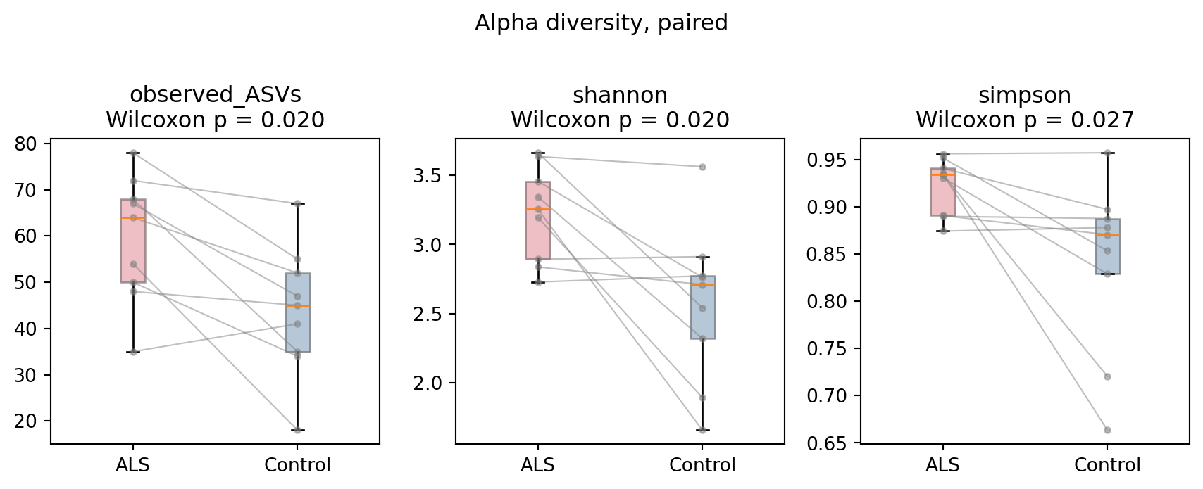
# Alpha diversity
Within-sample diversity is compared within matched pairs (paired Wilcoxon signed-rank
test). These metrics are computed from the ASV count table and do not depend on the
taxonomic classifier.
```{python}
#| lst-label: lst-alpha
#| lst-cap: "Compute three alpha-diversity metrics per sample and test them within matched pairs."
def shannon(c):
    """Shannon diversity index for one sample's ASV counts."""
    p = c/c.sum(); p = p[p>0]; return float(-(p*np.log(p)).sum())

# Three complementary within-sample diversity metrics, one row per sample.
alpha = pd.DataFrame({
    "observed_ASVs": (counts>0).sum(axis=0),         # richness: how many ASVs are present
    "shannon":       counts.apply(shannon, axis=0),  # richness and evenness combined
    "simpson":       1-(rel**2).sum(axis=0),         # chance two reads are different taxa
}).join(meta.set_index("sample")[["status","pair"]])

# Compare each ALS sample against its own spouse control (paired Wilcoxon signed-rank test).
rows=[]
for m in ["observed_ASVs","shannon","simpson"]:
    a = alpha[alpha.status=="ALS"].set_index("pair")[m]
    c = alpha[alpha.status=="Control"].set_index("pair")[m]
    a,c = a.align(c, join="inner")   # line up each ALS sample with its matched control
    rows.append((m, round(a.mean(),2), round(c.mean(),2), round(stats.wilcoxon(a,c).pvalue,3)))
astats = pd.DataFrame(rows, columns=["metric","ALS_mean","Control_mean","wilcoxon_p"])
astats
```
```{python}
#| label: fig-alpha
#| fig-cap: "Alpha diversity by group, paired. Gray lines join each ALS patient to their spouse control. ALS communities are more diverse on all three metrics."
# One panel per metric: a box per group, with gray lines connecting each matched pair.
fig, axes = plt.subplots(1, 3, figsize=(9, 3.5))
for ax, m in zip(axes, ["observed_ASVs","shannon","simpson"]):
    bp = ax.boxplot([alpha[alpha.status==g][m].values for g in ["ALS","Control"]],
                    tick_labels=["ALS","Control"], showfliers=False, patch_artist=True)
    for patch, gname in zip(bp["boxes"], ["ALS","Control"]):
        patch.set_facecolor(colors[gname]); patch.set_alpha(0.35)
    # Connect each ALS patient to their own control, so the within-pair shift is visible.
    piv = alpha.pivot_table(index="pair", columns="status", values=m, observed=True)
    for _, r in piv.iterrows():
        ax.plot([1,2], [r["ALS"],r["Control"]], color="gray", alpha=.5, lw=.8, marker="o", ms=3)
    p = float(astats.loc[astats.metric==m,"wilcoxon_p"].iloc[0])
    ax.set_title(f"{m}\nWilcoxon p = {p:.3f}")
fig.suptitle("Alpha diversity, paired", y=1.02); fig.tight_layout()
plt.show()
```
ALS communities are significantly more diverse than their matched controls (@fig-alpha):
observed ASVs and Shannon diversity, p = 0.020; Simpson diversity, p = 0.027.
# Beta diversity
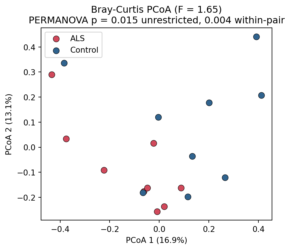
Between-sample structure is summarized with Bray-Curtis dissimilarity, tested by a
permutational analysis of variance (PERMANOVA, 9,999 permutations) and visualized by
principal coordinates analysis. The PERMANOVA is implemented directly here, following
@anderson2001permanova, and uses the fixed random seed set above. Because the design is paired,
the test is run two ways: with unrestricted permutation of group labels, matching the
original study, and with permutation restricted to within matched pairs, which respects
the paired structure.
```{python}
#| lst-label: lst-permanova
#| lst-cap: "Bray-Curtis PERMANOVA from scratch, with unrestricted and within-pair permutation."
# Bray-Curtis dissimilarity between every pair of samples, from their relative abundances.
samps = counts.columns.tolist()
X = rel.T.values; n = len(samps)
BC = np.zeros((n,n))
for i in range(n):
    for j in range(n):
        BC[i,j] = np.abs(X[i]-X[j]).sum() / (X[i]+X[j]).sum()
grp = meta.set_index("sample").loc[samps,"status"].values

def pseudo_F(D, labels):
    """PERMANOVA pseudo-F: between-group distance relative to within-group distance,
    computed from a distance matrix D and a grouping (Anderson 2001)."""
    labels = np.asarray(labels); uniq = np.unique(labels); N = len(labels); a = len(uniq)
    sst = (D[np.triu_indices(N,1)]**2).sum()/N; ssw = 0.0   # total sum of squares
    for g in uniq:                                          # within-group sum of squares
        idx = np.where(labels==g)[0]; ng = len(idx); sub = D[np.ix_(idx,idx)]
        ssw += (sub[np.triu_indices(ng,1)]**2).sum()/ng
    return ((sst-ssw)/(a-1))/(ssw/(N-a))

F = pseudo_F(BC, grp)   # observed statistic for the real ALS/control grouping

# Significance by permutation: how often does a reshuffled grouping match or beat F?
# (1) Unrestricted: shuffle the labels freely, matching the original study's approach.
cnt = 1
for _ in range(9999):
    if pseudo_F(BC, rng.permutation(grp)) >= F: cnt += 1
pval = cnt/10000

# (2) Within-pair restricted: only swap ALS/control labels inside a pair. This respects the
# paired design and is the more appropriate test here.
si = {s: i for i, s in enumerate(samps)}
pair_members = [(pairs.loc[p,"ALS"], pairs.loc[p,"Control"]) for p in pairs.index]
cnt = 1
for _ in range(9999):
    lab = np.array(grp)
    for a_s, c_s in pair_members:
        if rng.random() < 0.5:                              # flip this pair's labels with prob 0.5
            ia, ic = si[a_s], si[c_s]; lab[ia], lab[ic] = lab[ic], lab[ia]
    if pseudo_F(BC, lab) >= F: cnt += 1
pval_paired = cnt/10000

print(f"PERMANOVA (Bray-Curtis, pseudo-F = {F:.3f}):")
print(f"  unrestricted permutation (as in the original study): p = {pval:.4f}")
print(f"  within-pair restricted permutation (paired design):  p = {pval_paired:.4f}")
```
```{python}
#| label: fig-pcoa
#| fig-cap: "Principal coordinates analysis of Bray-Curtis dissimilarity. ALS and control samples separate along the first axis, consistent with a significant community-level difference."
# Classical (metric) MDS of the Bray-Curtis matrix: double-center, then eigendecompose.
J = np.eye(n)-np.ones((n,n))/n; B = -0.5*J@(BC**2)@J
ev, evec = np.linalg.eigh(B); o = np.argsort(ev)[::-1]; ev, evec = ev[o], evec[:,o]
pos = ev>0; coords = evec[:,pos]*np.sqrt(ev[pos]); varexp = ev[pos]/ev[pos].sum()*100  # % variance per axis
fig, ax = plt.subplots(figsize=(5,4.5))
for g in ["ALS","Control"]:   # plot the two groups in their assigned colors
    idx = [i for i,s in enumerate(samps) if grp[i]==g]
    ax.scatter(coords[idx,0], coords[idx,1], c=colors[g], label=g, s=60, edgecolor="k", lw=.5)
ax.set_xlabel(f"PCoA 1 ({varexp[0]:.1f}%)"); ax.set_ylabel(f"PCoA 2 ({varexp[1]:.1f}%)")
ax.set_title(f"Bray-Curtis PCoA (F = {F:.2f})\nPERMANOVA p = {pval:.3f} unrestricted, {pval_paired:.3f} within-pair"); ax.legend()
fig.tight_layout(); plt.show()
```
The ALS and control communities differ significantly (@fig-pcoa): unrestricted PERMANOVA
p = 0.015, matching the original study's approach, and the within-pair restricted test,
appropriate to the paired design, is stronger at p = 0.004. As with alpha diversity, this
result is computed from the count table and is independent of the classifier.
# Differential abundance
Taxa are collapsed to each rank, with any ASV below the 0.5 confidence threshold flagged
as unclassified, and compared within pairs (paired Wilcoxon test, Benjamini-Hochberg
false discovery rate per rank). Because the V4 model assigns 99 percent of reads at genus,
many genera can be tested.
```{python}
#| lst-label: lst-diffabund
#| lst-cap: "Helpers to collapse ASVs to a taxonomic rank and test each taxon within pairs."
def rank_table(rank):
    """Sum ASV counts to one row per taxon at the given rank; low-confidence calls are pooled
    into a single '(unclassified)' row rather than dropped."""
    lab = tax[f"{rank}_predicted"].copy()
    lab[tax[f"{rank}_raw_score"] < CONF] = "(unclassified, score < 0.5)"
    return counts.groupby(lab).sum()

def rank_rel(rank):
    """The rank_table counts expressed as per-sample percentages."""
    t = rank_table(rank); return t/t.sum(axis=0)*100

def diff_abund(rank, min_mean=0.1):
    """Paired Wilcoxon test of ALS versus control for each taxon above a minimum mean abundance,
    with Benjamini-Hochberg FDR correction across the taxa tested at this rank."""
    relt = rank_rel(rank).drop(index="(unclassified, score < 0.5)", errors="ignore")
    rows=[]
    for taxon, r in relt.iterrows():
        a = pairs["ALS"].map(r).astype(float).values       # ALS percentages, one per pair
        c = pairs["Control"].map(r).astype(float).values   # matched control percentages
        if max(a.mean(), c.mean()) < min_mean: continue    # skip vanishingly rare taxa
        p = 1.0 if np.allclose(a-c,0) else stats.wilcoxon(a,c).pvalue
        rows.append((taxon, a.mean(), c.mean(), a.mean()-c.mean(),
                     np.log2((a.mean()+1e-3)/(c.mean()+1e-3)), p))   # log2 fold change, pseudocount added
    res = pd.DataFrame(rows, columns=["taxon","ALS_mean_pct","Control_mean_pct",
                                      "diff_pct","log2FC","p"])
    if len(res): res["FDR"] = stats.false_discovery_control(res["p"])   # correct for multiple testing
    res["taxon"] = res["taxon"].str.replace(r"_\d+$", "", regex=True)   # drop GTDB numeric IDs
    return res.sort_values("p").reset_index(drop=True)
```
## Class
```{python}
#| lst-label: lst-class
#| lst-cap: "Differential abundance at the class rank (top six by p-value)."
diff_abund("class").head(6).round(3) # six most-different classes, ALS versus control
```
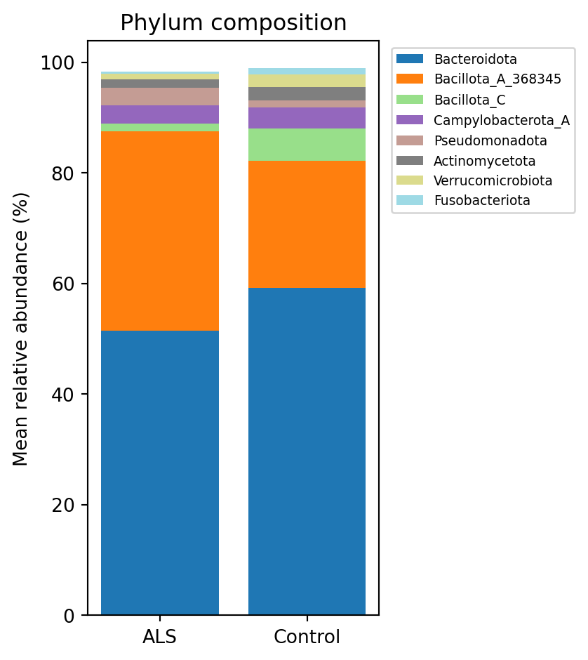
Clostridia, the dominant Firmicutes class, is enriched in ALS (36.0 versus 23.0 percent of
reads, p = 0.027), as is Gammaproteobacteria; Negativicutes trends in the opposite
direction. The same signal appears at the phylum rank as Bacillota_A (@fig-phylum).
```{python}
#| label: fig-phylum
#| fig-cap: "Mean phylum composition by group. ALS communities carry proportionally more Firmicutes (Bacillota) and less Bacteroidota than their matched controls."
# Take the eight most abundant phyla (plus the unclassified pool) and stack their group means.
relp = rank_rel("phylum")
top  = (relp.drop(index="(unclassified, score < 0.5)", errors="ignore")
            .mean(axis=1).sort_values(ascending=False).head(8).index.tolist())
comp = relp.reindex(top+["(unclassified, score < 0.5)"]).dropna(how="all")
mean_by = pd.DataFrame({"ALS": comp[als].mean(axis=1), "Control": comp[ctl].mean(axis=1)})
fig, ax = plt.subplots(figsize=(4.5,5)); bottom = np.zeros(2)
cm = plt.cm.tab20(np.linspace(0,1,len(mean_by)))
for k,(t,row) in enumerate(mean_by.iterrows()):   # stack each phylum on top of the previous
    ax.bar(["ALS","Control"], row.values, bottom=bottom, label=t, color=cm[k]); bottom += row.values
ax.set_ylabel("Mean relative abundance (%)"); ax.set_title("Phylum composition")
ax.legend(bbox_to_anchor=(1.02,1), loc="upper left", fontsize=7); fig.tight_layout()
plt.show()
```
## Genus
```{python}
#| lst-label: lst-genus
#| lst-cap: "Genera differing nominally (p < 0.05) between ALS and control."
g = diff_abund("genus")
g[g.p < 0.05].round(3)   # keep only the nominally significant genera
```
The ALS-enriched genera are members of the Lachnospiraceae and related Clostridia
(*Agathobacter*, *Blautia*, *Dorea*, *Mediterraneibacter*, *Acetatifactor*,
*Hominicoprocola*), together with *Parasutterella*. *Agathobacter* is a well-known
butyrate producer. As shown in the SILVA validation above, all of these except
*Acetatifactor* and *Hominicoprocola* are confirmed by an independent classifier; those
two remain DeepTaxa-specific. The genus-level differences are nominally significant but do
not survive false discovery rate correction at nine pairs (FDR about 0.34), so they are
hypothesis-generating rather than confirmed.
```{python}
#| lst-label: lst-prevotella
#| lst-cap: "Per-pair summary for Prevotella and Phocaeicola, including how many pairs run each way."
def genus_summary(prefix):
    """Summarize one genus (matched by GTDB name prefix) across the nine pairs: group means and
    medians, the number of pairs in which ALS is lower, and the paired Wilcoxon p-value."""
    gr = rank_rel("genus")
    s  = gr.loc[[i for i in gr.index if str(i).startswith(prefix)]].sum(axis=0)   # pool GTDB variants
    a  = pairs["ALS"].map(s).astype(float).values
    c  = pairs["Control"].map(s).astype(float).values
    return pd.Series({"ALS_mean_pct": round(a.mean(),1), "ALS_median": round(np.median(a),1),
                      "Control_mean_pct": round(c.mean(),1), "Control_median": round(np.median(c),1),
                      "ALS<Control pairs": f"{int((a<c).sum())}/9",
                      "wilcoxon_p": round(stats.wilcoxon(a,c).pvalue,3)})
pd.DataFrame({g: genus_summary(g) for g in ["Prevotella","Phocaeicola"]}).T
```
*Prevotella*, the dominant genus of the control microbiomes, is markedly depleted in ALS
(18.2 versus 43.8 percent; median 12.9 versus 57.6 percent), the same large effect the
original study reported. *Phocaeicola* moves in the opposite direction.
# Firmicutes-to-Bacteroidetes ratio
```{python}
#| lst-label: lst-fb
#| lst-cap: "Firmicutes-to-Bacteroidetes ratio per sample, tested within pairs."
pc   = rank_table("phylum").drop(index="(unclassified, score < 0.5)", errors="ignore")
firm = pc.loc[[i for i in pc.index if i.startswith("Bacillota")]].sum()   # Firmicutes = GTDB Bacillota*
bact = pc.loc["Bacteroidota"] if "Bacteroidota" in pc.index else pd.Series(0, index=pc.columns)
fb   = (firm/bact)                                                        # F:B ratio per sample
a = pairs["ALS"].map(fb).astype(float).values; c = pairs["Control"].map(fb).astype(float).values
print(f"F:B ratio  ALS median = {np.median(a):.2f}  control median = {np.median(c):.2f}  "
      f"ALS greater in {(a>c).sum()}/9 pairs  paired p = {stats.wilcoxon(a,c).pvalue:.3f}")
```
The bulk Firmicutes-to-Bacteroidetes ratio is not significantly different. In GTDB the
Firmicutes split into Bacillota_A (Clostridia, higher in ALS) and Bacillota_C
(Negativicutes, higher in controls), and the two offset each other. The Clostridia enrichment is a specific
class-level difference that the bulk ratio does not capture.
# Functional prediction (PICRUSt2)
The original study's strongest functional claim was that ALS patients lacked
butyrate-metabolism genes. We tested this by predicting gene content from the ASVs with
PICRUSt2 2.5.2 [@douglas2020picrust2] (mean nearest-sequenced-taxon index 0.124, no ASVs
dropped).
```{#lst-picrust .bash lst-cap="Predict gene-family content from the ASVs with PICRUSt2."}
# PICRUSt2 gene-family prediction (16 threads)
picrust2_pipeline.py -s asv_seqs.fasta -i asv_counts.biom -o picrust2_out -p 16
```
Butyrate genes are present in all 18 samples, with only a weak, non-significant trend
(@tbl-butyrate):
| Gene (KEGG orthologue) | Route | ALS | Control | Direction | p |
|---|---|--:|--:|:--:|--:|
| K00929 (*buk*) | Kinase | 2626 | 4372 | ALS lower | 0.16 |
| K00634 (*ptb*) | Kinase | 2318 | 4214 | ALS lower | 0.16 |
| K01034 (*atoD*) | CoA-transferase | 881 | 546 | ALS higher | 0.43 |
| Sum of butyrate orthologues | - | 9096 | 11883 | ALS lower | 0.30 |
: Predicted butyrate-pathway gene abundances (paired Wilcoxon). {#tbl-butyrate}
There is at most a weak hint of reduced butyrate-kinase-route capacity in ALS, but the
dominant CoA-transferase route trends the other way and total capacity is only about 23
percent lower (p = 0.30). The claim of a complete absence is not recovered here. This is the
most fragile comparison on either side, as it rests on a taxonomy-to-genome inference;
only shotgun metagenomics would settle it.
# Comparison with the original study
| Finding | Original study | This reanalysis (DeepTaxa) | Outcome |
|---|---|---|---|
| Alpha diversity higher in ALS | Chao1 p = 0.03, Shannon p = 0.004 | observed and Shannon p = 0.020, Simpson p = 0.027 | Consistent here |
| Community-level difference | PERMANOVA p = 0.002 | PERMANOVA p = 0.015 | Consistent here |
| *Prevotella* depleted in ALS | adjusted p = 0.002 | 18.2 versus 43.8 percent, p = 0.109 | Same direction, large effect |
| ALS lacks butyrate genes | PICRUSt prediction | present in all samples, weak non-significant trend | Not recovered here |
: Comparison with the original study's testable findings. {#tbl-reproduction}
Two of the original study's three testable findings are recovered here (@tbl-reproduction), in the
same direction and now resting on classification that an independent reference confirms; with nine
pairs they are consistent rather than conclusive. The functional butyrate claim is not recovered
under PICRUSt2.
# Summary
- DeepTaxa assigns a genus to 99 percent of reads at high confidence (mean 0.985).
- An independent SILVA classification confirms this is not merely confidence: the two
methods agree on the genus of about 94 percent of reads, and the genera underlying the
clinical findings are confirmed, except for *Acetatifactor* and *Hominicoprocola*, which
SILVA leaves unresolved.
- ALS gut communities are more diverse and structurally distinct from spouse controls;
both results are independent of the classifier and are consistent with the original study.
- ALS is enriched in Clostridia and Lachnospiraceae and depleted in *Prevotella*; the
genus-level differences are suggestive (nominal p < 0.05) but limited by nine pairs.
- The bulk Firmicutes-to-Bacteroidetes ratio and the claim of absent butyrate metabolism
are not supported in this reanalysis.
The diversity and community-level findings are consistent across methods but limited by the
nine-pair cohort; the genus and functional layers are hypothesis-generating at this sample size.
# References
::: {#refs}
:::